Which Excel Function Averages Cells In A Range Based On A Specified Condition?

Bottom Line: Learn to alter the formatting of an unabridged row of data based on the value of i of the cells found in that row.

Skill Level: Intermediate

Video Tutorial

Download the Excel File

If yous'd like to download the same file that I apply in the video so you can meet how it works immediate, hither it is:

Provisional Formatting Based On Jail cell Value.xlsx (138.7 KB)

Format an Entire Row Based on a Cell Value

Sometimes our spreadsheets can exist overwhelming to our readers.  Peculiarly when yous have a large canvas of data with a lot of rows and columns.  The reader needs to run into all the data, only nosotros also want to draw attention to some rows based on a condition.

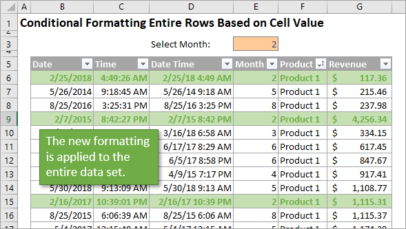
In this week's post, I answer a question from Dawna, a member of ane of our preparation programs.  She wanted to highlight the entire rows in a information set up when the value in a cell in the row matched a value in a cell exterior the table.

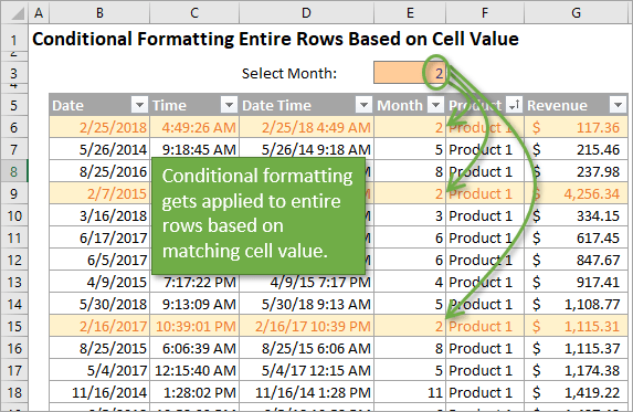
For this scenario, we can utilise Conditional Formatting.  This is a great feature of Excel that brings life to our spreadsheets and makes them much easier to read.

Conditional formatting also makes your files dynamic and interactive.  The user can rapidly alter the cell that contains the criteria and the matching rows will be highlighted.

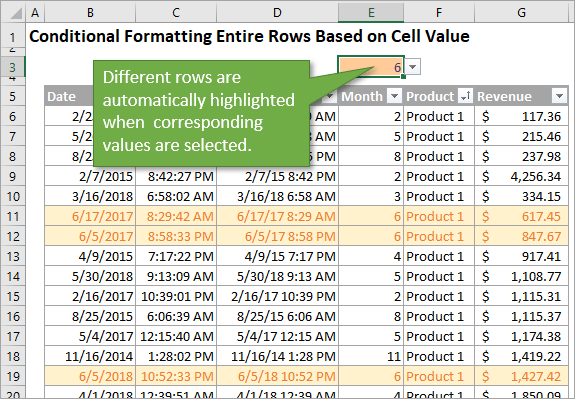
In the image higher up I changed the value in cell E3 to 6. All rows that comprise a 6 in column East are immediately formatted with the font & fill up color I specified in the conditional formatting dominion.

Conditional formatting is a fun characteristic that your dominate and co-workers volition love. Permit'south become information technology set!

Setting Up the Conditional Formatting

The video above walks through these steps in more item:

1. Showtime by deciding which column contains the data yous want to be the basis of the provisional formatting. In my example, that would be the Month column (Column E).
2. Select the cell in the commencement row for that column in the tabular array. In my case, that would be E6.
3. On the Dwelling tab of the Ribbon, select the Conditional Formatting drop-downward and click on Manage Rules…. That will bring up the Conditional Formatting Rules Manager window.
4. Click on New Rule. This will open up the New Formatting Rule window.
5. Nether Select a Rule Blazon, choose Use a formula to decide which cells to format.
6. Under Format values where this formula is true, you lot are going to write a very simple formula. The formula should prepare the jail cell that yous desire the provisional formatting applied from equal to the kickoff cell in the column that you already identified in Step one. So in our example the formula would read =$East$3=$E$half-dozen.
7. To ensure that the conditional formatting applies to all of the rows in the table, we need to change the absolute relative referencing. In other words, we are going to remove that dollar sign in front of the 6 in our formula. You lot tin can either manually delete it, or you tin can striking F4 twice to attain this step.
8. Click on the Format… push button to choose whatever format options you like. You tin alter the font, the fill, the border, etc.

Your New Formatting Rule window should look something similar this:

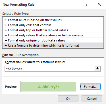
Conditional Formatting Rule

Once you striking OK, you lot will be taken back to the Conditional Formatting Rules Manager window. Hither y'all will meet the rule that you lot only created.

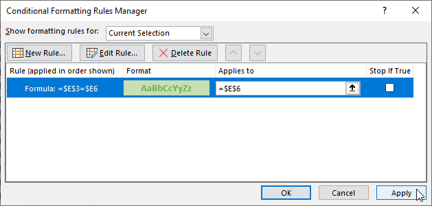
Y'all can click on Employ, merely at this betoken the rule will but be applied to cell E6 because that is the prison cell you started from and it is what's listed in the Applies to field. Nosotros want to extend this rule to the whole table.

To do that, click on the icon to the right of that field (information technology has an upward facing arrow) and select the range of the entire table. In the case, this would be the data ranging from B6 to G1002 (=$B$6:$Grand$1002).

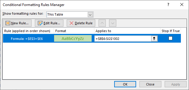
Click Use one more fourth dimension and the new formatting applies to the entire data fix.

Using Other Comparison Operators

The rule that you create doesn't e'er take to set a value equal to (=) another value. You can change the format for rows that are

• less than (<),
• less than or equal to (<=),
• greater than (>),
• greater than or equal to (>=),
• or not equal to (<>)

any specific value. And it doesn't take to be a number. Information technology can be text, dates, or other data types every bit well.

It doesn't matter which of those comparison operators you use. The conditional formatting is just applied based on whether your logic statements are true or fake.

If you'd similar to get a better understanding of logic statements, as well as IF functions, I recommend this tutorial:

IF Role Explained: How to Write an IF Statement Formula in Excel

The sample file also uses a drib-down listing (data validation list) in prison cell E3. Check out my article on How to Create Drop-downwards Lists in Cells – Information Validation Lists to larn more.

Conclusion

I hope this is helpful to you. If you lot have any questions almost the process, please leave them in the comments. You lot can also leave any suggestions or recommendations you might accept on the topic.

Thanks!

Source: https://www.excelcampus.com/tips/conditional-formatting-rows-cell-value/

Posted by: phillipsentlead.blogspot.com

Share this post